Contents:
- FOXS Placental Morphology
2. Case Report: Fetal squames (vernix) in uterine veins with postpartum uterine atony
3. Continuing review of Dynamic Modeling textbook
4. Review of umbilical cord coiling index (not included here since it already has a page on the blog).
FOXS Project: Placental morphology
This FOXS project proposes a system approach to explain why a failure of fetal oxygenation often does not have a direct anatomic causation, and why it can occur suddenly and unexpectedly in mothers with the same risk factors. The question most relevant to me as a pathologist is why infants with similar placental diagnoses and clinical histories can have such different outcomes e.g. stillbirth, perinatal HIE or normal uncomplicated deliveries. The review in LOOP of system dynamics will explain how parameter differences can have major effects on unstable equilibrium points. Our conventional diagnoses of the placenta may not be giving the needed information to understand these vital parameters. Parameters in the placenta might be the efficiency of oxygen transfer if maternal flow is decreased, or the maximal amount of oxygen that can diffuse in a period of time. These parameters would modify variables in equations of oxygen transfer in the placenta.
For this essay, I want to consider placental pathology only in its role in failure of fetal oxygenation. As a pathologist, I receive placentas from infants having suffered stillbirth or perinatal hypoxia. They often show diagnostic lesions, but those lesions are not visibly different than similar lesions in a perfectly uncomplicated pregnancy. In these cases, without a clear anatomic or clinical cause of fetal death, the explanation is logically due to one of three things: 1) Clinical events that are separate from the anatomic diagnosis, although possibly associated. 2) A less severe form of the same anatomic lesion, for example a 20 % premature placental separation compared to a 90%, and 3) Differences in placental reserve, that is of the capacity of the placenta to maintain fetal maternal oxygenation if there is compromise of the fetal or maternal circulation. Consider an example of each of these possible explanations.
For the first case, different clinical events with the same placental lesion, consider a pregnancy with some kind of umbilical cord compromise such as a functional short cord or a cord trapped alongside the fetal head. Contractures of the uterus lead to intermittent partial occlusion of the umbilical cord blood flow. These intermittent occlusions lead to lesions of fetal vascular malperfusion in both placentas. In one case, the cord blood flow occlusions are longer and more complete and lead to progressive fetal acidosis which causes stillbirth or fetal hypoxia. (See my website, www.obstetricpathology.com, for discussions of experimental umbilical flow occlusion in sheep and of the effects of fetal acidosis in general in Dr. Ron Myers primate experiments.) In another case, the flow occlusions fall below a threshold in which progressive lactic acidosis occurs, and the blood oxygen recovers after each occlusion. The first infant is stillbirth and the second has a normal birth. Both have a placental diagnosis of lesions of fetal vascular malperfusion (FVM) from the intermittent umbilical cord occlusion1,2. These FVM lesions, when not due to local causes such as villitis or to fetal thrombophilia, implicate compromised fetal blood flow, but not whether that compromise was causing progressive acidosis. It is possible that specific features of FVM lesions may be more predictive of a cause of fetal circulatory compromise that is at higher risk for acidosis and death, but that remains to be discovered.
For the second case, differences in quantitative lesions, consider abruption. I reviewed premature placental separation of the placenta (abruption) as a cause of stillbirth and found that at least 50% of the placental volume was separated from the maternal blood supply in stillbirth3. A similar sensitivity to loss of functioning placenta also appears to be true with placental infarctions and with placental villitis of unknown etiology. These lesions, like premature placenta separation, reduce the amount of residual functioning placenta. Even in these three lesions, the effect on placental function (and hence fetal hypoxia) may depend on several other factors such as the rapidity of the destructive onset of the lesion (a slower onset could allow for an increased development of new villous function), on the overall mass of functioning placenta in relation to the metabolic need of the fetus (roughly equivalent to fetal weight), or on the prior functional adaptations of the villi.
For case 3, the idea of placental reserve is an old idea but not easy to determine in anatomic pathology practice. The extent of a placental lesion is usually presented in terms of the percent of the placenta involved, or the number of villi with the lesion. Yet, equally important to placental functioning, may be the total amount of remaining, functioning placenta. A small placenta relative to the fetal oxygen requirement will suffer more from a 50% premature placental separation than a large placenta which will have more functioning placenta left after a 50% loss. More difficult to measure is the functional state of that remaining placenta. If the placenta has chronically adapted to low maternal blood flow, a sudden decreased fetal blood oxygen level may not be able to extract as much oxygen as would a previously normally perfused placenta. Different placental morphology may have different capacity to increase fetal oxygenation depending on the cause of an episode of hypoxia, for example a decrease in umbilical cord perfusion versus a decrease in maternal intervillous perfusion.
We cannot completely evaluate the entire volume of placenta but must rely on sampling to determine 1) the total functional placental volume and 2) its specific functional morphology. First consider determining the functional volume of placenta. The total weight of the drained, unfixed placenta with the cord and membranes removed is often used as a rough proxy for the volume. More rarely volume is determined by displacement in a liquid, or approximately calculated from the measured geometry. A ratio of the placental weight to the birthweight then provides a rough indication of functional placental tissue per gram of fetus. This ratio demonstrates that some placentas even in uncomplicated pregnancies are smaller or larger than expected. However, the placental weight is not a reliable measure of functional placenta because: 1) it has a variable amount of retained fetal and maternal blood, and non-placental mass, e.g. a variable amount of perivillous fibrinoid and fibrin, and 2), it fails to account for the diseased non-functional placental mass e.g. villitis. Microscopic findings can be used to correct for these variables. However, more difficult to measure is the different functional growth patterns of the villi that reflect different functional ability to transport oxygen or permit intervillous blood flow. This is reflected in morphologic lesions such as delayed or accelerated villous maturation, but these diagnoses are not sufficiently quantitated to measure their effects on fetal oxygen transfer. Clearly, getting accurate measures of the functional reserve of the placenta is going to be a multistep procedure to quantitate and adjust for all of these confounding factors.
Assuming a sampling protocol that provides a reliable picture of the all the functioning villi in the placenta, what anatomic features will provide measures of villous function? The villi are a branching system starting with a thick primary stem that branches into generations of progressively thinner stem villi that end in terminal villi. Between the stem and terminal villi are intermediate villi with functions of both. The stem villi conduct fetal blood to the terminal villi. They have more collagenous stroma, and the arteries and veins have a similar diameter with a thick muscular media (Fig 1).

Figure 1 The pale pink branching structures are the conductance villi with large muscular veins and arteries. (2x)
They are not rigid but provide some protective structural strength. It is likely that the muscular media of the vessels evolved to control matching of fetal circulation to maternal blood flow. Vascular control is demonstrated with both loss of fetal blood flow, as with fetal bypass for experimental heart surgery in sheep causing an intense rise in placental vascular resistance4, and of maternal blood flow with placental infarction causing an abrupt cessation of local villous blood flow. Growth of conductance villi can be from both lengthening and increased branching. Possibly the relative muscular thickness of fetal vessels, and total cross-sectional area of conductance vessels at different levels of the villous branching may be measures of the ability of the placenta do decrease or increase fetal placental blood flow.
The terminal villi have two opposing functions in relation to oxygen. Thinned areas over bulging capillaries provide the thin barrier thickness that promotes oxygen diffusion, which is relatively slow, analogous to capillary alveolar areas in the lung5. In the placenta these are called vascular-syncytial membranes (Fig 2). In contrast, areas with thick syncytiotrophoblast are not only a physical barrier to diffusion of oxygen from mother to fetus, but also consume high amounts of oxygen along a microvillous border involved in active transport of nutrients, analogous to intestinal function (Fig 3). With maturation of villi over gestation more of the terminal villous surface area develops vascular syncytial membranes presumably to meet increasing oxygen demands of the larger fetus. The oxygen diffusion capacity depends on the total surface area of perfused vascular syncytial membranes.
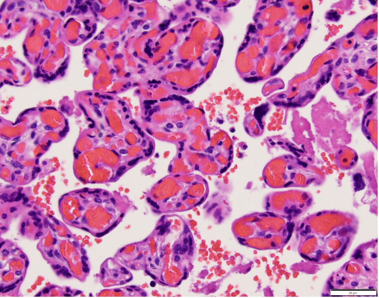
Figure 2 Thinned syncytium over capillaries, vascular syncytial membranes (arrows), provide a thin barrier to permit oxygen diffusion between maternal and fetal blood
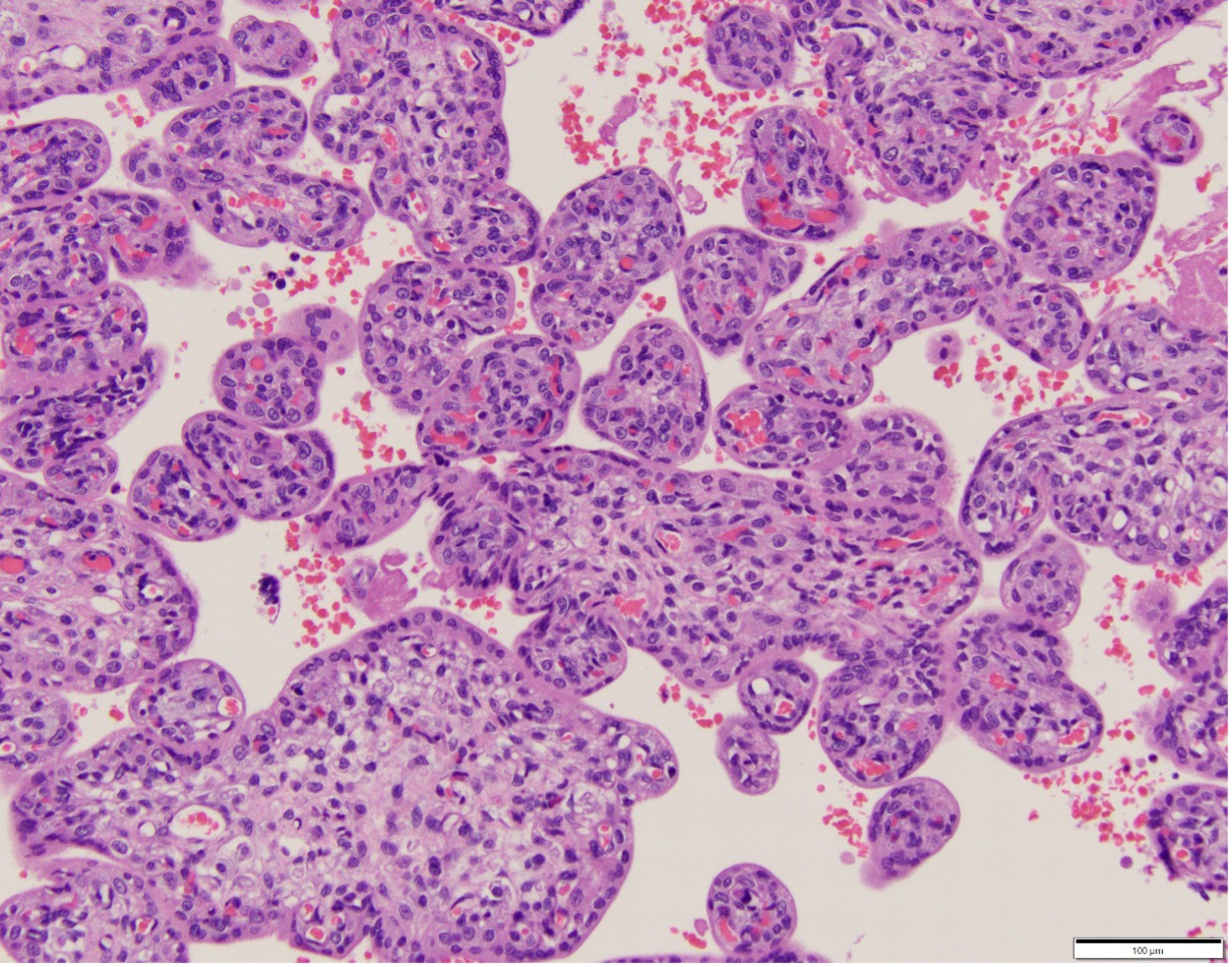
Figure 3 In this younger gestation placenta, an outer thick syncytial trophoblast layer and, more central capillaries is designed for active nutrient transfer.
The last problem is the resistance of the intervillous space to maternal perfusion. This could be a critical value to fetal survival with a decrease of maternal blood pressure. The remodeled spiral arteries entering the intervillous space have lost their smooth muscle and have a fixed, wide diameter that lowers vascular resistance and increase the flow at normal blood pressures (Fig 4).
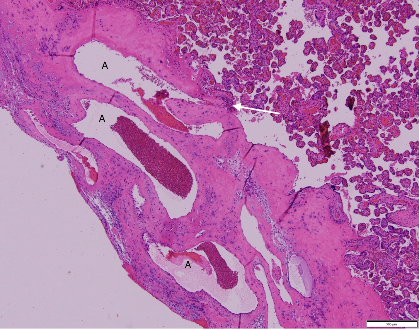
Figure 4 The arrow points to the opening of the spiral artery into the intervillous space. The spiral artery “A” has a wall of fibrinoid and cytotrophoblast, the muscle have been removed in the cytotrophoblast remodeling.
The angiograms of placental circulation of monkeys, which have placentas with a similar structure to humans, show blood enters from the spiral arteries and circulates like a fountain6. The resistance beside the linear distance from the base to the fetal surface of the placenta is going to occur because of the obstruction by villi and by fibrinoid/cytotrophoblast barriers. In general, the villi are sparser at the entry of the spiral artery, and this structural adaptation becomes more prominent over gestation, or in cases of pathologically low placental perfusion. To maintain needed flow during maternal hypotension, the resistance needs to be low enough to still permit sufficient maternal blood flow. Calculating this resistance from the morphology will be a challenge, perhaps analyzing streamlines.
The computer assisted villous analysis from digitized images can follow one of two methods: 1) A specific tissue identification similar to previous stereological studies, e.g. teaching the computer to recognize placental tissue components and selecting filters to identify features e.g. vascular syncytial membranes based on barrier thickness between the outer border of syncytiotrophoblast and the adjacent capillary border. Statistical tools can adjust for the 2 dimensions of a microscope slide to 3D surface areas, and the total surface area of vascular-syncytial membranes on the microscope slides can be projected from the multiple samples to the whole volume of functioning placenta. The computer identifications can often be verified by a pathologist. 2) A hands-off approach that compares digital slides with the relevant clinical diagnosis of fetal oxygenation failure, i.e. stillbirth, perinatal asphyxia, or Cesarean section because of non-reassuring fetal heart tones, to controls matched for gestational age and birthweight. A training set is provided to the computer, then the computer classifies new cases as either fetal oxygenation failure or normal. This approach requires a very large number of cases, cannot “explain” the basis of the computer decision, but could provide new insights. There are hybrid techniques that fall between these two approaches.
A brief aside, finding causation in placental pathology is of necessity postpartum, or even postmortem. The value of doing so is to improve understanding and suggest better hypothesis for clinical testing and therapy. To make this project meaningful, clear communication between pathologists and clinicians is crucial. The goal is to synthesize clinical and pathologic observations, as well as basic science studies, to optimize clinical treatment and reduce failures of fetal oxygenation. This newsletter needs input from different perspectives, so please submit your thoughts.
Addendum: placental sampling proposal
A proposed protocol to measure the total volume of placenta and its various functional capacities as a research tool with the understanding that it is based on my experience, but not validated. In a way this protocol is a test of the hypothesis that these measures of functional placenta may explain some otherwise unexplained causes of fetal oxygenation failure.
Gross measuring
- Obtain an image of the fetal surface, with a ruler in the image. Then using software, available with some digital slide viewers, measure 1) the total surface area of placenta including accessory lobes, and 2) the diameters of chorionic surface arteries and veins around the umbilical cord insertion before they branch. There is some evidence that the spread (widths) of a placenta is functionally important. Chorionic surface vascular diameters vary from placenta to placenta. Whether this variation is due to chronically different flow rates, or to acute constriction of surface vessels in not known. One hypothesis is that it may be a measure of residual fetal blood in the placenta, but from experience, it does not seem correlated with delayed cord clamping.
- Obtain an image of the maternal surface. Using software measure the depressions from retroplacental hematomas. A separate experimental protocol will investigate inking spiral artery and decidual vein ostia to determine the distribution per area of placental base.
- Sever the membranes and cord, and remove any loose adherent clots, or cyst fluid. Weigh the placenta.
- Cut the placenta in even 1 cm slices, lying them with the same surface up and then obtain an image, again with a ruler. I have made the cuts using an electric meat slicer, or manually with a long-bladed knife. There are other commercial food slicers that may be more accurate and safer.
- Using software, manually determine the area of the slices or use machine learning, and then calculate the volume. Again manually or with machine learning, subtract gross lesions from that volume, including infarctions, focal massive perivillous fibrinoid, or pale areas from avascular villi or villitis. The suspect areas are labeled and sampled for microscopy to confirm the gross diagnosis. Create a graph of the height of the placental slices, and of the size and distribution of lesions. The height of the placenta could affect the response to a decrease of pressure in a maternal inflow to the intervillous space.
- Parenchymal samples are taken as usual and placed in cassettes. Attempt to have a sample from fetal to maternal surface in one cassette, but if not possible, the sample can be divided to have the fetal and maternal halves in labeled cassettes. Choosing these samples requires a non-random approach. In stereology the idea would be to have a true random sample without consistent orientation. A true random sample would lose information, for example the change in villous characteristics from fetal to maternal surface, and the variability from one placentome to the other. A placentome is the volume of placenta perfused by a spiral artery which can vary because of differences in blood flow in different spiral arteries. Another source of variance that is difficult to account for is the lack of exact relationship between the incoming spiral artery flow and the alignment of a primary stem villous system coming from the fetal surface. The initial approach would be to take 2 cm wide samples from fetal to maternal surface of normal appearing parenchyma, starting at the first non-marginal slice, and obtaining a sample from every slice, but shifting the distance from the margin 4 cm to obtain staggered samples. The slices are labeled consecutively, and that label identifies the samples from that slice. A relatively large sample is needed not only to see adaptation of placentome flow, but also to better estimate the extent of microscopic pathology that is not necessarily evenly distributed within the parenchyma. Adjacent to these vertical samples, slices just above and parallel to the base and just below and parallel to the fetal surface will be put into a cassette also labeled by slice. These slices will be used to count respectively spiral arteries and primary villi entering the intervillous space per area.
- Analysis of the samples with machine learning will attempt to make corrections to the gross volume to determine the actual functional volume of placenta and to evaluate whether variability between samples indicates that fewer sample are adequate, or more are needed.
1. Redline RW. Clinical and pathological umbilical cord abnormalities in fetal thrombotic vasculopathy. Hum Pathol 2004;35(12):1494-8. (http://www.ncbi.nlm.nih.gov/entrez/query.fcgi?cmd=Retrieve&db=PubMed&dopt=Citation&list_uids=15619208).
2. Khong TY, Mooney EE, Ariel I, et al. Sampling and Definitions of Placental Lesions: Amsterdam Placental Workshop Group Consensus Statement. Arch Pathol Lab Med 2016;140(7):698-713. DOI: 10.5858/arpa.2015-0225-CC.
3. Bendon RW. Review of autopsies of stillborn infants with retroplacental hematoma or hemorrhage. Pediatr Dev Pathol 2011;14(1):10-5. (In eng). DOI: 10.2350/10-03-0803-OA.1.
4. Lam CT, Sharma S, Baker RS, et al. Fetal stress response to fetal cardiac surgery. Ann Thorac Surg 2008;85(5):1719-27. DOI: 10.1016/j.athoracsur.2008.01.096.
5. Mayhew TM, Jackson MR, Haas JD. Microscopical morphology of the human placenta and its effect on oxygen diffusion: a morphometric model. Placenta 1986;7:121-131.
6. Ramsey EM, Donner MW. Placental vasculature and circulation. Philadelphia: W. B. Saunders Company Ltd, 1980.
Case Report # 2 Vernix caseosa and thrombi in uterine veins in postpartum uterine atony.
Clinical history: This G3P2 mother at 41 weeks of gestation underwent a Cesarean section for arrest of fetal descent following complete cervical dilatation with 3 hours of pushing and a Category 2 fetal heart rate pattern. A low transverse uterine incision was made that extended laterally to the uterine vessels. The membranes were ruptured at the Cesarean section. A 4,070 g infant with Apgar scores of 9/9 at 1/5 minutes was delivered. The extended incision was closed achieving hemostasis, and a small laceration on the posterior uterus was sutured. The uterus remained atonic after the usual therapies, and a Jada suction device could not keep up with the bleeding. Total maternal blood loss was estimated at 5.5 liters with massive transfusion needed. Her blood pressure dropped to 80s/40s with pulse 120-130. The sutured incision began to rebleed. A Cesarean hysterectomy was performed, during which a cervical laceration was also found.
Pathology: The gravid uterus demonstrated the sutured low transverse incision, a sutured low posterior laceration, and a hemorrhagic cervix (Fig 1). The uterus was bivalved, demonstrating a wide cavity with an area of hemorrhage on the posterior wall. Microscopically, the posterior uterine slides demonstrated numerous thrombi with embedded fetal squames and surrounding acute inflammation (Fig 2,3).
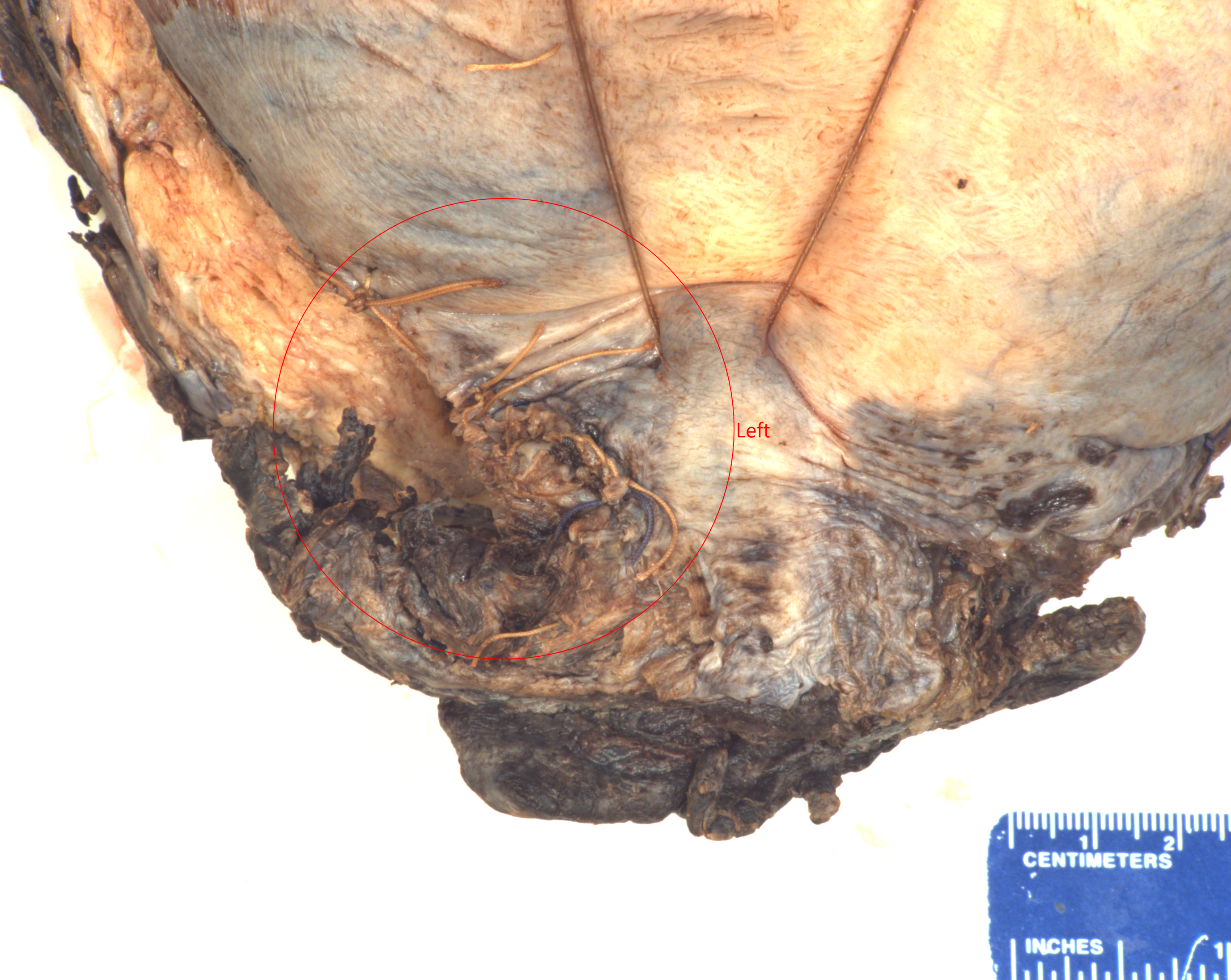
Figure 1 The sutured area is the posterior repair area that demonstrated the veins with squames and thrombi
.

Figure 2 Low power of the large myometrial veins with a central thrombus and vernix accumulation (H&E)

Figure 3 Higher magnification of the accumulation of vernix in the upper left corner, and scattered fetal squames to the right. (H&E)
Abduction (forming hypothesis on incomplete evidence): The most plausible route of the vernix into the uterine veins was through the posterior wound that seemed to extend from the low transverse anterior incision. The membranes were ruptured during the Cesarean delivery, and fluid could have been sucked into the large decidual veins by negative venous pressure. That the vernix would cause thrombi is not surprising, although I do not know if this has been reported. The maternal hypotension was attributed to the blood loss, but it is possible that amniotic fluid also entered the veins causing a small amniotic fluid embolism that contributed to the hypotension.
The difficult hypothesis is to state that the vernix associated thrombi caused the uterine hemorrhage and atony. The venous distribution would have delivered amniotic fluid to the uterine and ovarian veins, and it seems unlikely that it could have caused more widely distributed thrombi or a local consumption coagulopathy sufficient to cause persistent hemorrhage. On the basis of a maternal autopsy that I did decades ago, one hypothetical path of causation is that the vernix trigger ed a pelvic vein thrombus and increased uterine venous pressure. Fig 4 shows the ovarian vein thrombus from the autopsy, which continued to an inferior vein thrombus. The mother died days after delivery from a pulmonary embolus. To my surprise, the ovarian thrombus was filled with fetal squames (I no longer have images of the microscope slides). At my suggestion, the mother in this current case had a scan, which failed to demonstrate pelvic thrombi.
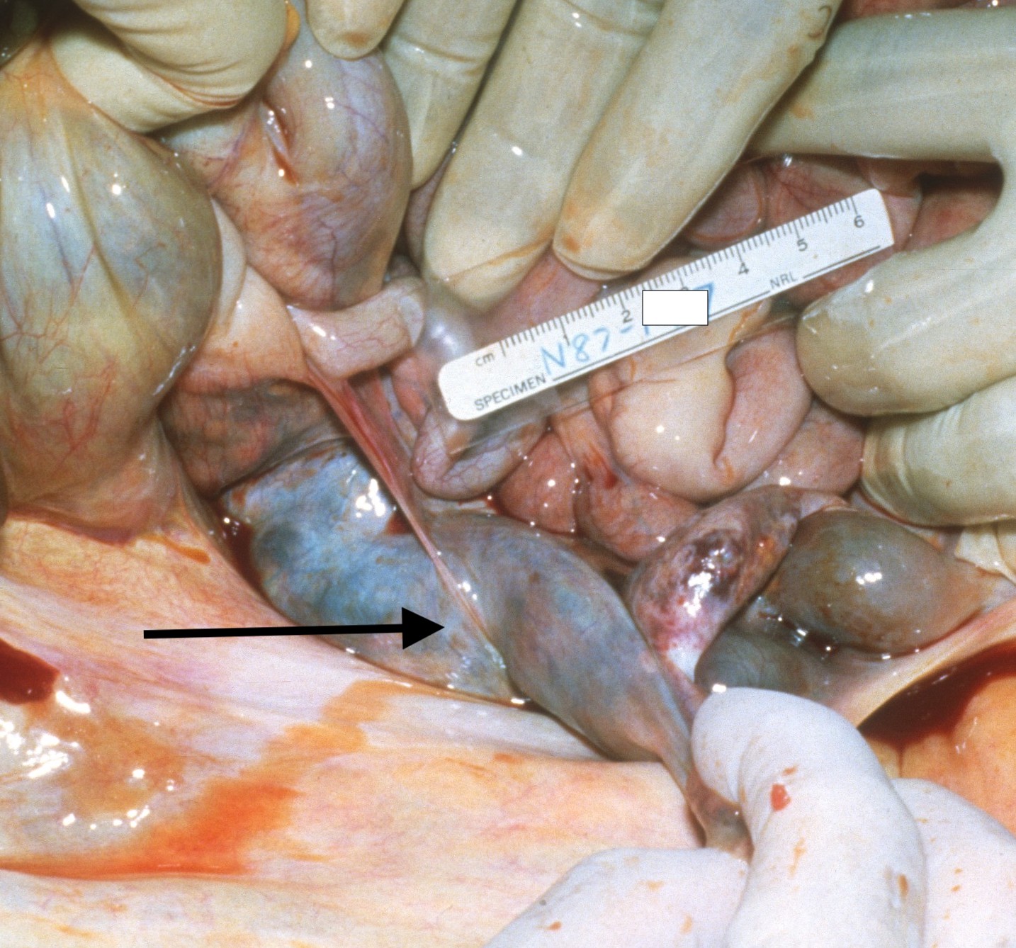
Figure 4 The arrow points to the large ovarian vein thrombus that had intermixed fetal squames
A reported series of 34 cases of postpartum hemorrhage of unknown etiology, i.e. excluded any possible preexisting risk of PPH, 15 controls from C/S, and another 18 postpartum controls (unclear how obtained) found increased uterine neutrophils, monocytes, and mast cells1. They used a tryptase stain that produced a halo around degranulating mast cells which showed more cells with halos in the cases. These findings could have been a secondary reaction. However, they then identified anti-coproporphyrin (as a marker for meconium) staining in myometrial blood vessels in 24 of the cases (70%) and none in controls. This was interpreted as indirect evidence that amniotic fluid with meconium had circulated in the myometrial vessels.
Now the adductive hypothesis is that amniotic fluid can be more widely distributed in the uterus, perhaps by uterine contractions after delivery, and that the fluid, or meconium in the fluid, degranulates mast cells and this causes the uterine atony.
There is not a lot of supportive medical literature for this hypothesis. I can confirm from a study I did of gravid uterine biopsies at the Cesarean incision (unpublished) that mast cells are plentiful in the pregnant myometrium (Fig 5). (This is the only image that I ever scanned. The rest are destroyed. It is not the best demonstration) I am not aware of the physiologic function, if any, of this accumulation. However, it is not a huge stretch to suggest that triggering them to release histamines, bradykinin etc., might favor smooth muscle relaxation.

Figure 5 This toluidine blue stained thick section for electron microscopy shows numerous dark stained cells in the interstitium that are the mast cells whose granules show metachromasia with the stain.
I think it is worth looking in gravid uteri for venous squames and thrombi as evidence of vernix injection to determine the frequency of this finding and whether it is associated with unexplained uterine atony. The special tryptase stain for mast cell degranulation or for immunohistochemistry of coproporphyrin for meconium are not routinely available.
1. Farhana M, Tamura N, Mukai M, et al. Histological characteristics of the myometrium in the postpartum hemorrhage of unknown etiology: a possible involvement of local immune reactions. J Reprod Immunol 2015;110:74-80. DOI: 10.1016/j.jri.2015.04.004.
My notes on Modeling Live: The mathematics of Biological Systems. A. Garfinkel, J. Shevtsov, and Y Guo, Springer 2017.
These are just my notes. I may have things wrong, but it would be useful (I hope mutually) to have feedback if anyone else is using this book to understand dynamic systems in biology.
The book starts out with a familial ecological system, a very simplified version of predator and prey where the predator eats prey, which allows the predators to increase, but the prey decreases, then the predators don’t have enough prey to eat, which reduces the number of predators, allowing the prey numbers to increase, which then allows the predators to increase because there is more prey. The authors point out that this simplified system ignores many details, like weather fluctuations, disease breakout, plant abundance and many other things. This is a starter model, which is what we need to create for the relationship between fetal oxygen delivery and fetal oxygen consumption. The placenta sends oxygen to the fetus, the fetus consumes it, lowering the oxygen that returns to the placenta, the placenta then increases the oxygen, returning oxygen to the heart.
The goal is to translate systems like predator prey relationships, but also into many others, into a mathematical model. The book starts with a simple time series that can be obtained by observation of the number of prey and the number of predators over time. From the book.
To make this system reflect a fetal oxygenation system, we can relabel shark numbers to the fetal blood O2 level, and the tuna number to the cardiac output using “fetal heart rate” as a proxy (at least within narrow limits). Fetal O2 utilization will decrease blood O2 which will by chemoreceptor/adrenergic reflex, increase cardiac heart rate, which will then increase O2 extraction from the placenta. That oxygen will be utilized by the fetus, thus returning to the beginning of the cycle.
The authors use this shark tuna example to show how this cycle relies on a positive and a negative feedback loop. A positive feedback loop increases a positive value and decreases a negative value (makes it more negative). A negative feedback loop decreases a positive value and increases a negative value (makes it less negative). Tuna to sharks is a positive loop: More tuna, more sharks which leads to a negative loop: More sharks, less tuna. They don’t make it explicit, but it takes two cycles to create the time series oscillation, as the then less tuna leads to less sharks as part of the return to the positive feedback loop, and in the second return to the negative feedback loop, less sharks leads to more tuna, and then the process repeats.
The text goes one step further with a section: Counterintuitive Behaviors of Feedback Systems. In real systems, there are multiple feedback loops such as the reproductive rate of the sharks and fish, etc. Removing most of the sharks in this system at a point in the cycle can unintuitively result in a stable increase in sharks.
The most obvious lesson here is that our model of fetal oxygenation needs to be a lot more complex to approximate reality and when we have it, there may be unexpected changes in response to a change in a system variable. Also, some system models will be better models of reality than others.
Section 1.2 Goes over basics of functions, maps the independent (input) value to the output (dependent) value, can be e.g. a table or a formula e.g. F(y) = 2x, or any other mapping as long as there is a single output value for each input value. X2 = Y2 is not a function since there are 2 values X = 2, and =-2. Not all functions can be written as a formula. For the shark tuna time series there is no formula for the graph. The important point for us is that for the overwhelming majority of biological models there is no known formula for the time series.
The input values that a function can accept is the domain. That domain is often all real numbers R, or all positive R+ numbers, with the restriction that the domain cannot result in division by a zero. In real world systems it is important to choose domains the make physical sense.
Section 1:3 States and State Spaces
The state of a system is the value of the state of quantitative variables at a given point in time. One of the hardest parts of building a model is deciding on the variables. Each state variable can have only one value at a given time, that is each is a function of time.
The state space is the set of all conceivable values of a system. Usually these are continuous variables, even if they don’t make sense, e.g. 3.1 rabbits. If they are not continuous, then a different kind of modeling is needed.
For a one variable system, the system state is a point on a line (its state space) at a given time. For example, fetal venous oxygen level would be a value on the line segment from 0 to the limits of the
Systems can have multiple values, and the values can be added if they are the same, apples to apples, and they can be multiplied by a scalar. They can also be graphed. For example, a two variable system can have its states plotted on an X, Y axis. For our system Maternal fetal (M, F )space would plot M, maternal PaO2 on one axis, and F, fetal Pa O2 on the other axis. Time is not plotted on the graph. But the point from one state to the next over time creates a vector The length of the vector is a scalar quantity, and the vector is the slope (in a single point a slope from 0,0 to M,F
Most models work with many variables, creating vectors in n- space. A single variable can be described as point on a line, two variables as a point on a plane, and three variables as a point in 3D space, but higher dimension space is more difficult to represent graphically. Vector addition and scalar multiplication still work the same way in n-space, as long as the variables have the same number of components, so for a = (a1….an) and b = (b1…bn) then a + b = (a1 + b1 ,…, an + bn). For multiplication c(a1,…, an) = (c a1,…,c an). Change is in a state space is movement of the variable values over time (t) in the space, e.g. from PaO2 = 80 at t1 to PaO2 = 30 at t2.
1.4 Modeling change
A model embodies a set of hypotheses about the causes of change in a system.
The state variables can be considered as levels or stocks, that is a number, and the rate of change in these variables are the flows. That rate of flow may depend on the level of the variable. The textbook uses a simple example of water flow into and out of bathtub. The rate of outflow varies directly with the level of water, that is the higher the level the faster the outflow which is a linear relationship of pressure to flow. The actual slope of the curve depends on the constant from the outflow pipe diameter. The relationship of fetal oxygen level to rate of flow of oxygen in from the placenta or out to the fetus is more difficult to isolate. However, it is clear that the level of oxygen effects many rates that tend to maintain the oxygen level like shunting blood away from non-vital organs or increasing cardiac output by increasing heart rate.
The variables being modeled in the system collectively make up the state of the system and hence are referred to as state variables.
Expressed as a word equation: change in stock = input flows – output flows. The equation does not need both input and output.
Equations of this kind do not have a term for the level at any time. They only consider the rates of change, but this leads to a powerful way of modeling.
This can be confusing, but is clarified as models are converted to mathematical equations.
A sample model for a one state variable X (the number of animals) system is discussed. X’ is the rate of change of X, so X’ = birth rate – death rate.
Obviously not a complete model, so the authors make another key statement: All models make huge assumptions, and it is critical to be able to state what they are for a given model.
They then simplify birth rate to each animal has 0.5 births per year given as b, which is multiplied by the number of animals, bX and similarly for death rate to X’ = bX – dX
Simplify to (b-d) X = rX, of course this does not describe a useful relationship, because other factors than the inherent birth and death rate influence the X’ like predators, crowding (available food), etc. So they had a crowding factor that X’ is bX * crowding factor. They define a carrying capacity as k and X/k as the fraction of the carrying capacity already in use, which then leaves (1- X/k) available resource.
This is called the logistic equation X’ = bX (1 – X/k)
It was not clear to me why this is a multiplication until they derive it based on probability, basically drawing 2 aces from a deck is the probability of drawing one ace squared, or in this case perhaps 2 rabbits landing on the same cabbage which is proportional to the square of the number of rabbits or number of cards in the deck. The trick is to then make X’ = bX – cX2, if that proportionality constant c is b/k then we can factor out bX and we are back to X’ =bX(1-X/k). I have notes scribbled all over this page (31) and folded the corner. Taking the time to follow it is worthwhile, as variants will keep showing up. It limits the possible rate of change by the population. If X becomes larger than k then the (1-X/k) will become negative and birth rate will fall. If k is larger than X , then (1- X/k ) will be positive and the population will grow, (If equal the growth rate will be 0)
Two variable systems: The text presents several two variable systems where the change of a variable depends on the level of another. One example is a mass on wheels attached to a spring. X’ = V and V’ = F/m (this is just a reformatted F = ma , V’ is the derivative of a, but the book avoids that terminology.) Hookes law (which almost never holds in biology) F = -kX. Substitute got F V’ = -k/m X, then they set the units for k/m =1
Then V’ = X and X’ = V. They go one to add a friction component to the Force as an exercise. There are other exercises to write “change” equations for many different types of systems.
The section on “seeing change geometrically” is hard to duplicate with text, but is critical to understanding the illustrations of equilibria. Start with a state space that is a straight line, X’ = 0.2X, each value for X’ can be graphed as a vector on the straight line with a direction and a magnitude. They then plot the vectors on the line, lying equal portions of the vector centered on the value for X, and calling it a useful fiction. This is a bit strange, but in the fields with more dimensions this begins to make sense. This vector field is defined as the differential equation, change vector (X’), corresponding to every state point X. The authors use color differences to differentiate the state space (X) from the vector space (X’). The vectors then plotted on the state space, in this case a line, obviously can’t all be plotted since each state point X has a vector often longer than a point, the vectors would overlap, so only some are plotted. The idea is to show the direction of change in X. A linear example is the logistic growth model equation X’ =rX(1-X/k). At X = k, the vectors change from right facing to left facing with that inflection point marked by a large dot, instead of a vector arrow. Next this concept is used to graph the vectors (as very short arrows or arrow heads) with 2 variables. The authors suggest using the program SageMath to plot the vectors, which I downloaded but have not yet gotten to work. They plot the Lotka-Volterra predation model with the 2 variables predator and prey. The result is dizzying.
Another way to look at it is to plot the trajectory from an initial state to a different state (that is from an initial X0 to another X. Then only the vectors actually traversed are plotted, this trajectory is also referred to as the integral curve or the solution curve. The trajectory will be different with different initial points. This is a key diagram technique that the authors admit the learning to interpret them, requires time spent. Note they do not tell how fast the system changed only the direction. The graphs of a trajectory and a time series attached to each other are helpful, since the trajectory shows the direction and magnitude of change but not the actual value of the variable, while the time series shows the result of the change in the value of the variable. The illustration with two variables, are confusing, and I finally had to assume that only one variable was being used in the time series.
Aside from learning to visualize the graphics of the trajectory of a state, the authors emphasize that the vector field is a function that assigns the state point of the system to state vectors. This means that there is exactly one change vector for each point in state space. Because they are functions, the vectors cannot cross or touch one another. The surprising result is that if we know a systems state at any time we can find its trajectory for all time.
The chapter on trajectories ends with two questions: Is there a single trajectory through a given change point that everywhere follows the change arrows. The answer is yes based on the Picard-Lindelöf theorem, which states that if our differential equations are well behaved (not defined in detail in text, just that the equations in the text will meet those criteria) then there is a unique curve through any given point that follows the change vector at that point. The second question is can we find the equation for that trajectory. The answer is almost never. The curve of course is changing continuously and requires calculus to calculate the curve. This is great if there is great when there is a solution when the change in time goes from delta t to 0. However, almost none of the curves encountered in biology can be solved! However we can plot the trajectory graphs using Euler’s method.
Euler’s method is just to choose a very small delta t (change in time) , and keep solving using that very small delta t and adding it to the previous value, creating an approximation of the trajectory. (this is a sort of calculus approach only instead of an infinitesimal change the calculation just keeps solving directly for a very small change. The Sage computer program recommended in the textbook uses a more accurate version of Euler’e method, but it is not needed to understand the more complicated math. The computer curve looks smooth and is a good approximation to a true solution.
They break Euler’s method down into 5 steps
- Start from point X0
- Evaluate X’ at X0. We will call this X’0.
- Multiply the change vector X’0 by the small number
t
- Add
- Repeat steps 1 through 4 for the point X1 to get X2, keep repeating.
Considering the core of this chapter, basically plotting the first derivative of a variable against the variable. The problem conceptually is that you can’t physically plot a vector with a scalar and a direction as a point. However, to be able to see how the X variable is changing over time within a system, it is a needed visualization. If we look at a simple model that yields exact solution with calculus, such a throwing a ball upward, we know the initial position, we know the velocity as a vector in space. Using Newton’s equations we know exactly how gravity is decreasing the velocity, and for each point of time we can calculate exactly how high the ball is. We can take any point on a plot of that height and knowing the starting conditions, there is only one answer because we know the velocity (and the second derivative showing how the velocity is changing. Thus knowing the initial position of the starting point on a graph of the height versus the derivative (velocity vector), we can see that the variable will change over time as it follows the solution of the adjacent derivative equation. A similar concept would be true of a population change, although there is no continuous solution to the change equation (the equivalent in calculus to the derivative). We can still use the change equation to find the variable value at the next point in time, but we do this by approximating a curve using “short” intervals.
Even in the Newton ball throwing, we could not plot the changing velocity vector on every point. On a flat 2 D graph. What is being done in the graphs is that the plot shows selected points with a direction and a scalar length for the change equation. The plot not only specifies the value of the variable, say population of an animal, but also where the animal is on the solution to the derivative at that same point in time. The value of the variable depends on initial conditions as well as the change equation, and that is what the vector is plotting. After a period of time, the equation is re-solved, and that new value of X is moved along the graph based on solutions of that change equation, which uses the previous value of X and adds on the new solution. When you throw a ball, based on the initial conditions and Newtons law of motion, you know exactly where it will be at any time and if we plotted the changing velocity vector between 2 points in time (think the change in velocity (scalar and vector) you would see on the distance versus time series plot, exactly where the ball will be at that new time.
If we start with the same value for the variable, but with different initial conditions, the path will not be the same, but would start at a different point on the graph, and travel along the change equation from that point which would not be the same trajectory. If a ball is thrown at 45 mph at 45 degrees to the horizon, it will not follow the same trajectory as a ball thrown at 15 mph at 30 degrees to the horizon. The value of the height above the ground would be different for both balls, but with the same change (differential) equation. The difference is that the values in the equation, namely the starting velocity (gravity is a constant), would be different. That is the best I could do with it, but maybe someone else can clarify better. (To be continued)
